

Foreword
I wrote the following many years ago when I learning basic statistics. It still serves as a reference occasionally and I thought I’d put it online. There is also a page on Statistics – Confidence Intervals.
Arithmetic Mean
The arithmetic mean, or average, is calculated simply by summing individual values in a list, and dividing by the number of values.
If the list contains all possible values, then the list is a statistical population and the mean is called a population mean or true mean and is often designated by the symbol μ, which can be calculated precisely by:
μ = 1/N * (a1 + ... + aN) = 1/N * ∑ai   where i = [1, N]

Equation 1a
Population Mean
where N is the number of values in the population.
In practice, however, it is usually impossible to know all possible N values because populations are typically continuous in nature, and therefore, the number of possible values infinite. However, it is possible to estimate the population mean by drawing n random samples from a larger population of N possible values. The estimation is known as the sample mean, because it is the mean of the sample, rather than the population.
In this case, we can write:
ā = 1/n * (a1 + ... + an) = 1/n * ∑ai   where i = [1, n]

Equation 1b
Sample Mean
The difference between equations 1a and 1b is subtle, but it is important to recognise that the sample mean ā represents an estimate of population mean μ, and that the larger the number of samples n taken, the closer the sample mean approximates the population mean μ.
With regard to performance testing, we can say that the number of measurements (N) which we could potentially observe is infinite*, but in practice we can only sample a finite number (n). Therefore, a mean value of such measurements will provides us with an estimate (ā) of the system’s true performance (μ), and the more measurements made–the more accurate the estimate will be.
* Strictly speaking, due to numerical precision restrictions, the number of measurements made with computers are possibly finite, but very large nevertheless.
The distribution of a population (i.e. the possible values) describes the probability of observing (or measuring) any value within a specific range. Many natural phenomenon exhibit, what is referred to as, a normal or Gaussian distribution.
In a normal distribution, it is most expected to observes values close to the population mean, while values far from the mean are expected less often. For example, if a population mean is estimated to be 10, values such as 9.8, 9.9, 10.1 etc. may be observed frequently, while values such as 3 or 17.5, while possible, may be seen infrequently.
The shape of a normal distribution is shown below.
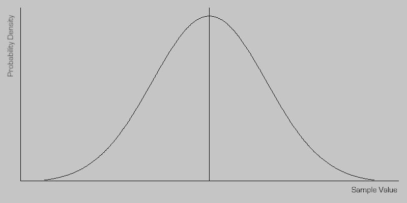
Note that a normal distribution peaks at the mean μ and is symmetrical.
Central Limit Theorem
The Central Limit Theorem states that if the sum of the variables has a finite variance, then it will be approximately normally distributed. Since many real processes yield distributions with finite variance, this explains the ubiquity of the normal probability distribution.
The Central Limit Theorem implies that if the sample size n is “large,” then the distribution of the sample mean is approximately normal. Of course, the term “large” is relative. Roughly, the more “abnormal” the basic distribution, the larger n must be for normal approximations to work well. The rule of thumb is that a sample size n of at least 30 will suffice.
It is important to understand that the Central Limit Theorem refers to the distribution of the sample mean, not the distribution of data itself. However, the normality of the sample mean is of fundamental importance, because it means that we can approximate the distribution of certain statistics (i.e. standard error), even if we know very little about the underlying sampling distribution.
Variance
The variance of a random variable (or somewhat more precisely, of a probability distribution) is a measure of its statistical dispersion, indicating how its possible values are spread around the expected value. Where the population mean shows the location of the distribution, the variance indicates the scale of the values.
The variance of a finite population of size N is given by:
σ2 = 1/N * ∑(ai - μ)2   where i = [1, N]

Equation 1a
Population Variance
This is known as population variance and represents the case where all possible values of the population are known, which is rarely the case.
More likely, the statistical population will be large, or infinite, and the calculation of the population variance impossible. In this case, it is possible to estimate the population variance by calculating a sample variance, as determined by drawing n samples at random from the larger (or infinite) population.
A source of confusion is that there two commonly used formulas for calculating sample variance:
sn2 = 1/n * ∑(ai - ā)2   where i = [1, n]
Equation 1b
Biased Sample Variance
or:
sn-12 = 1/(n - 1) * ∑(ai - ā)2   where i = [1, n]

Equation 1c
Unbiased Sample Variance
Here we are using “s2“, rather than “σ2“, to denote that the result is an estimate calculated only from a sample n, rather than the population N.
In addition, note the different “n” and “n-1” in the above equations. Equation 1b is equivalent to equation 1a, but the sample is treated as if it where the population, and the sample mean is used in place of the population mean. Whereas, equation 1c is known as the unbiased estimator of population variance, and is the method used by convention in applied statistics where the population size N is known to be large or infinite.
The results of both equations can be referred to as a sample variance, but will give slightly different results due to the different “n” and “n-1” terms. In practice, however, the difference becomes negligible as n becomes larger.
Standard Deviation
A more understandable measure of variance is called standard deviation–simply the square root of variance, as denoted by the symbol σ. As its name implies it gives, in a standard form, an indication of the possible deviations from the mean, as illustrated below for normally distributed data.
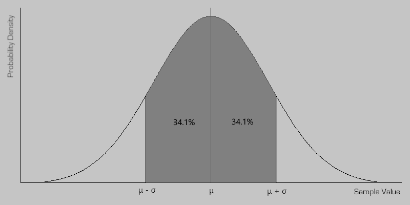
Normally Distributed Data
One often assumes that the data is from an approximately normally distributed population. If this assumption is justified, then one standard deviation (σ) equates to a range around the mean where the probability of observing a value is approximately 68.27%.
In addition, for normally distributed data, it is known that about 95% of the values are within two standard deviations of the mean and about 99.7% lie within 3 standard deviations. This is known as the “68-95-99.7 rule”, or “the empirical rule”.
The population standard deviation is defined by:
σ = √( 1/N * ∑(ai - μ)2 )   where i = [1, N]

Equation 2a
Population Standard Deviation
In practice the standard deviation must be estimated by calculating a value based up on a sample of the population, rather than the population itself. The result is known as the sample standard deviation, and as with variance, there are two commonly used formulas for calculating it:
sn = √( 1/n * ∑(ai - ā)2 )   where i = [1, n]

Equation 2b
Population Standard Deviation
and:
sn-1 = √( 1/(n - 1) * ∑(ai - ā)2 )   where i = [1, n]

Equation 2c
Sample Standard Deviation
Here we are using “s”, rather than “σ”, to denote that the result is an estimate calculated from a sample. Equation 2c is known as the sample standard deviation, and as with the equivalent unbiased estimator of variance, it is the method used by convention in applied statistics where the population size N is known to be large or infinite. Note, that it is not correct to refer to equation 2c as the “unbiased standard deviation”, as the ‘unbiasedness’ of the variance does not survive the square root term.
Pooled Standard Deviation
Pooled standard deviation is a way to find a better estimate of the true standard deviation given several different samples taken in different circumstances where the mean may vary between samples but the true or population standard deviation is assumed to remain the same. It is estimated by:
s = √( ∑( si*(ni - 1) ) / ∑(ni - 1) )   where i = [1, L]

Equation 3
Pooled Standard Deviation
where ni is the sample size of the i’th sample, si is the standard deviation of the i’th sample, and L is the number of samples being combined.
Arbitrarily Distributed Data
If it is known that the data is not normally distributed, or it is not known whether the distribution is normal or not, one can always make use of the Chebyshev Theorem to determine how much data lies close to the mean.
This states that, for any positive k, where k >= 1, the proportion r of data lying within k standard deviations of the mean is at least:
r = 1 - 1/k2

Equation 4
Chebyshev's Theorem
This holds true for any population no matter what the shape of distribution, and maybe taken to be a worst case for any scenario.
For example, for a population which is not normally distributed, we can be sure that at least the proportion 0.56 (or 56%) of the data lies within 1.5 standard deviations. Whereas, if we knew that we were dealing with a normally distributed population, it can be shown that 56% of the data would lie within only 0.77 standard distributions.
Standard Error
The standard error of a method of measurement or estimation is the estimated standard deviation of the error in that method. Namely, it is the standard deviation of the difference between the measured or estimated values and the true values. Notice that the true value of the measurement is often unknown and, this implies that, the standard error of an estimate is itself an estimated value.
Standard Error of the Mean
The standard error of the mean describes the probable error associated with the sample mean. It is a measure of how close the sample mean is likely be to the true or population mean.
The standard error of the mean is an estimate of the standard deviation of the sample mean based on the population mean. Given that a standard deviation equates to a 68.27% probability, we could say that the sample mean (an estimated value) is within +/-1 standard error of the population mean (true value) with a 68.27% level of confidence.
One method of standard error calculation would be to determine the sample mean multiple times using different randomly drawn samples, and then estimate the standard deviation around the mean of the means.
In practice, we do not need to estimate the mean multiple times as a statistical method already exists:
SE(ā) = s / √n

Equation 5
Standard Error of the Mean
where s is an estimate of the standard deviation as determined, for example, by equation 2c. Note that because s is an estimate, then it follows that SE(ā) is an estimate also.
The Central Limit Theorem implies that if the sample size n is “large,” then the distribution of the sample mean is approximately normal, irrespective of the distribution of the underlying data. Therefore, the standard error is not dependent upon an assumption that the population is normally distributed.
Standard Error of the Standard Deviation
As discussed, where the calculation of standard deviation is based upon a sample of a larger population, the result is an estimation. The standard error of the standard deviation gives the probable error associated with the sample standard deviation, and can be calculated by:
SE(s) = s / √(2n)

Equation 6
Standard Error of the Standard Deviation